How to Use Pivot Table in Excel in 2010

Pivot Table in Excel 2010: Hello Friends, Today We'll discuss how to Use a Pivot table in Excel 2010.  A pivot table is one of the powerful features of MS Excel. This tutorial will show you how to create a Pivot table in excel to summarize a set of the large dataset according to the requirement. Pivot table report reflects the different view on the same data. You can easily compare data by the Pivot table.For more easily you can also create a Pivot chart to display a summarized data at one place.

What is a Pivot Table?

A Pivot table is a report that summarizes,analyze and present a summary of spreadsheet data. It allows you to extract a significance or useful data from a large dataset. It is beneficial when you have a long list of data and basically used for analyzed countless spreadsheet records. We create a Pivot table according to the information and field it means which field to view and how the information should be displayed. There are mainly four things which we can perform using Pivot table in excel:

• Set up a large dataset in excel so that you can use for a Pivot table.
• Create a Pivot table with that data.
• Change the Pivot table report to display different views on same data.
• Drag,sort and Filter fields according to the requirement.

Steps for Insert a Pivot Table in MS Excel 2010

To insert a Pivot table in MS Excel follow some steps:

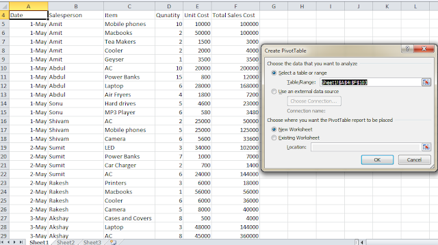
• Click any cell inside the large dataset.
• Then on the Insert tab, Click Pivot table. (A dialog box appears in which excel automatically select all the data then choose the location where you want the Pivot table report to be placed)

• Then click Ok.

Designing a Pivot Table Layout

For creating Pivot table Layout follow some steps:

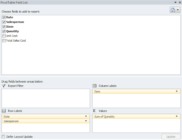
• When you create a Pivot table then you'll see Pivot Table field list.

• To create a layout of Pivot table, you first select the Fields then place them in the current location in the field layout area.
• Then Pivot table is generated according to the requirement as display below:

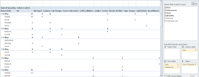
Here the Pivot table shows the total number of each product sold by each salesperson on each day.

Changing a Pivot Table

You can change a Pivot table to show the table in another way. For that you can follow some steps:

• Click inside Pivot table report then Pivot table Field list reappear.
• Change the layout of Pivot table according to the requirement.
• After these changes, you'll see some reflection on the same data in your Pivot table.

Here the Pivot table shows sold products down the side and name of the salesperson across the top.

How to Create a Pivot Chart

To create a Pivot chart follow some necessary steps:

• Click any cell inside the dataset.
• On the Insert tab, click Pivot table.
• Click OK.
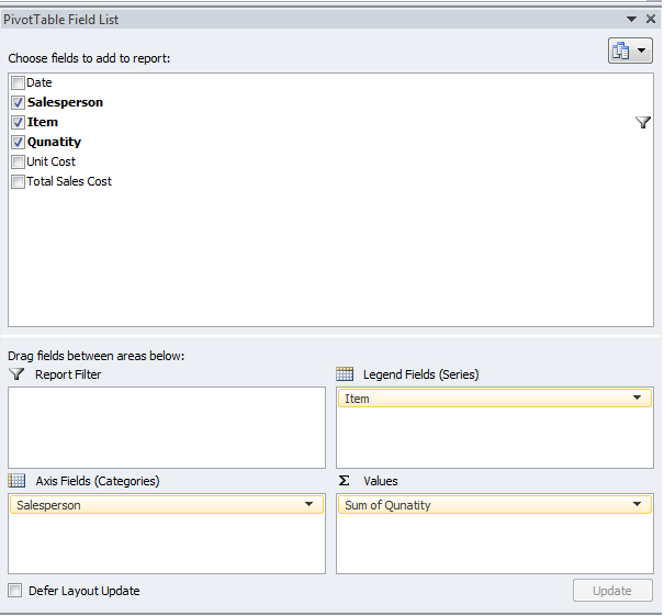
• You'll see Pivot table Field List, you have choose Fields to add to report and Drag fields between areas like report filter,Legend fields,Axis Fields,and the sum of values.

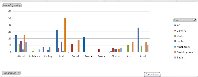
• Then Pivot chart is generated that is displayed below:

Here Pivot Chart shows the name of the salesperson and the quantity of sold item by each person.

Conclusion:

Thus,in this post, we'll discuss that how to use Pivot Table in Excel 2010. Pivot table provides the better way to find the useful information in a minimum time so this tool is very useful in business or in the large organization for prepare the report. If you like this post then you can share this post with your friends, colleagues, and relatives. You find an update on the regular basis. You can also share this post on facebook, twitter, Google+ or other social media website. If you find any issue regarding this post then you can write in the comment section. We'll revert back to you as early as possible.