Truckload Transportation - are you paying to ship air ?

How full is a "full" truck?   Not sure?  That's a shame, because when you contract for truckload freight, you pay for the whole vehicle, whether you fill it or not.   As I'll show you, the regulations around what constitutes "full" for weight are very complex.  In addition, the 3D jigsaw puzzle to pack product into the trailer space, distributing weight correctly and minimizing damage is exceptionally challenging.  Get it wrong and you are paying to ship air.  

It is much easier to plan to approximate rules or guidelines than to figure out what's really going on and it is common in the CPG industry to plan transportation loads based on these approximate rules.   Unfortunately, these approximate rules are very dependent on what you are trying to load (as well as who made up the "rule") so you will rarely encounter the same "rule" twice.  Typically what you will see is based on weight, pallet positions or cube.  Rules that restrict what's loaded to maximum limits like:

• 40,000 lbs of product
• 2,500 cubic ft of product
• 48 pallets of product.

None of these are right and they routinely result in shipping air.

Depending on the product and the vehicle,  I can safely, and legally, load much more than 40,000 lbs of product, (much) more than 2,500 cubic feet many more than 48 pallets.  

One particularly bad example I have encountered said "a truck is full when there is 38,000 lbs of product in it".  If I can find a way to, legally and safely load 45,000 lbs in the trailer it’s as though 7,000 lbs of product just shipped free, effectively saving 15% ((7,000/45,000 = 15.5%) in freight cost.

So, why is this so difficult to get right?  Let's look at the regulations around weight.

Weight Limits

If your product is "heavy", you will probably hit a weight limit in loading.  "Heavy" in this instance is roughly 20 lbs per cubic foot or more.  Much less than this and you will probably hit a space limit first (see below).

The government sensibly places restrictions on how heavy a loaded vehicle may be and how that weight must be distributed to be carried safely.   To get a feel for  the complexity involved, here is a link to the relevant page from the US Department of Transportation.  Stay just long enough to get confused then head back here :-)   Bridge Formula Weights 

To summarize (and simplify):

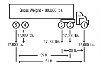
• The  total weight of the vehicle (including product, packaging, pallets, fuel, driver, etc...) must not exceed 80,000 lbs.
• There are limits for the weight on individual axles (shown below in this graphic from the US Department of Transport)

Note for the mathematically inclined:

If anyone is really interested in being able to calculate what weight should be on each axle given a particular layout of product in the trailer you need a little physics/engineering math.  Here is a great example of how a beam transfers load with an interactive calculator.

With the right math, you can calculate the center of gravity for the product and how that weight would be distributed to the axles.  Move the center of gravity forwards (e.g. by moving heavier product to the front) and you take weight of the rear wheels and transfer it to the tractor unit.  Quite how that weight then gets distributed to to axles 1 through 3 depends on where the "kingpin" connection (between the trailer and the tractor unit) is relative to the tractor units axles. You can build such a model in Excel.

So, can you plan to a total rig weight of 80,000 lbs?  No, sorry,  there are only so many options for how to layout product in the vehicle and there may be no layout that balances weight well enough across all axles to max out the 80,000 lb overall limit.You need to find the layout that gets closest to that limit and live with the loss.

Alternatively, you may run out of space in the vehicle before you get close to a weight limit.

Space Limits

If product is reasonably light (low density) we will probably be constrained by space before weight becomes a problem..

A reasonably standard trailer's internal dimensions are approximately

• 52' long
• 8' wide
• 8' (usable) height

That's a little over 3,300 cubic ft of space available to you.  However, you are typically loading with palletized product and you will not get to use most of this space.   Let's look at how well you can use the floor space first.

A standard pallet for US grocery is 40" wide, 48" long. The ability to fill the trailer floor-space depends a lot on how well these palletized units fit.  

If pallets will fit in the trailer "wide:wide" it's possible to put 30 pallet footprints in a 53' trailer.

If  the trailer is too narrow or product overhangs the pallet, you have to go to other configurations.   "Chimney stacking" maxes out at 28 footprints.

If you can't turn pallets at all, "narrow:narrow" loads max out at 26 footprints (although with any overhang on the pallets at all you will likely get 24/25)

In each case there is floor space you cannot use.  Load "narrow:narrow" and you have already lost almost 20% of the available space.

Now let's look at vertical space.  This is much more variation in the height of trailers and in the height of doors to those trailers.  If the door height is restrictive , perhaps because the door rolls up inside the trailer, that will limit the product you can get into that trailer.  Let's assume for now that we can safely get to 8' high. 

How much of the vertical space we can use depends on what we are loading.  Some product cannot be stacked, pallet on pallet, without causing damage.  Some pallets are too tall to allow anything (except an unusually short pallet) to fit stacked on top of it.  Very short pallets may be able to stack 3 or even 4 high.

If I assume 40" high palletized product, double stacked, we can use 80" of the 96" vertical space (83%).

Combine that with "narrow:narrow" loading and we max out a truck at 83% * 83% = 69% space utilization. From a "cube" standpoint the trailer is only 70% full and it's at capacity.  Hence rules like "the trailer is full at 2,300 cubic feet of product" when the trailer has over 3,300 cubic feet of air.

Depending on product dimensions and the ability to stack product we may be able to load much more than 2,300 cubic feet or much less.

Reducing Damage

We could spend a lot of time on this, but for now suffice to say, we would like to load the trailer so that product is less likely to get crushed, to move as the vehicle corners or to land in a heap at the front when the driver must, necessarily, brake.  This puts additional constraints on what product can go where in the vehicle, reducing, again, the weight you can carry and/or the volume you can load into the available space.

Equipment  limitations

If the pallet handling equipment (for either shipper or receiver) can't stack pallets or can't handle them turned, you will necessarily lose a lot of payload capacity.  Unless this is for very short trips where you can pay for the freight-cost with handling labor savings, you need to invest in warehouse equipment.

Not all trucks/trailers are the same.  By design they can be very different, tractor units weighing anywhere between 11,000 and 20,000  lbs.  Trailers can be vary by a few thousand lbs too.  Even equipment of the same make, model and year can be different depending on its setup (kingpin position) and the addition of aftermarket parts.  (Mount a new fuel tank too near the front and see it use up the limited capacity you have on the steering axle).  If weight is an issue for you, you will need to work with your carriers to understand what equipment they are bringing in.  Lightweight equipment is worth more to you, heavyweight equipment should be avoided or contracted at a low enough rate to offset the loss in carrying capacity..

Pulling it all together

Each of these sets of restrictions, weight, space, damage and equipment are complex: accurately modeling any of them is a challenge.  Depending on what you load: heavy or light product, slightly oversize, stack-able or not,  the factors that constrain you continually move.  And, beyond modeling it, you need to optimize: to find the selection and layout of product that maximizes your vehicle loading.

My Take

If you're lucky enough to have consistently-sized, palletized product with consistent low or high density that is consistently  stacked and loaded on consistent carrier equipment  you may be able to build a simple rule that really does max out your truck loading.  Good for you!   For the rest of us, such "rules" are poor guesses at best and can leave a lot of money on the table.  

You are NOT going to build this in Excel unless you have a lot of functional knowledge, very advanced skills in mathematical-optimization and the ability to program your own optimization code.  I have built a load optimization tool (It's a weakness, I like to know how things work).  I have also built my own tools for inventory-optimization, neural-network modeling, genetic-optimization, forecasting and many other needs..  Some of these tools are still in production use today, others were essentially learning opportunities.  In this instance, I chose to buy the software because it has richer functionality than what I chose to build myself.

(On a technical note, application-specific,heuristic optimization routines solve these problems well and quickly.  Mixed-Integer-Programming can get you most of the way, but personally I can't see how to embed some of the damage-reduction ideas into a linear objective function and as the heuristic works so well, you don't need the overhead or complexity of integrating a math programming tool) 

Any load building “optimizer” that asks you to specify a maximum weight or cube or number of pallets is really just automating these approximate rules rather than helping you truly max out the load.  An optimizer that is implemented as a stand-alone package is interesting but not really useful: you need this capability integrated into order-processing, deployment and transportation planning to be effective.  You need the right tool for the job.  These tools do exist, they work and it's not worth your time or effort to write them again.

There are a number of tools in the market that work in this space.  Google "load building optimizer" to see some.  I have not reviewed them all, far from it, but I can tell you that not all "optimization" is the same.  Having "optimize" in the sales literature does not mean it will do a great job for you or that any actual optimization is really taking place.

If you want a quick recommendation I suggest you talk to Transportation | Warehouse Optimization. they have a great load building tool and can extend this further into optimizing case-pick routing, pallet builds and shipping locations.

Let's assume you are doing a reasonably good job today without a load optimizer.  What would an extra 5% off your freight spend be worth to you?  Enough to invest in the right tool for the job?

A final thought

These rules-of-thumb can be very persistent.  Having implemented a system to drive increased payload coming out of one manufacturing site, I was perplexed some months later to see that the load factor had shrunk back to where it started.  It turns out that the warehouse supervisor at the plant was adjusting each and every load plan manually to fit with his interpretation of the “rules”.

Do you need daily Point of Sale data? Do you like selling more product?

Most people report on their Point of Sale data in weekly or perhaps even monthly buckets .  If you are interested in seeing a long-term trend or annual seasonality that's OK, but if you really want to know what's going on, to ensure you have product on shelf, and promotions running when your target shoppers are in store - you need daily POS data.  Don't believe me?  Let's look at an example...


I've created the data for this example so that there are no issues with confidentiality but not only does it closely represent reality, I have seen many more extreme versions of this in real data.

First let's look at 2 years of weekly Point of Sale (POS) data.  Anything interesting happening here?

I think we can say that there is no obvious seasonality, and there seems to be no trend in the data: longer term sales are neither  growing nor declining.  There appears to be no pattern to it: sales oscillate up/down in a fairly random looking manner,  sometimes, it's up or down for 2 weeks at a time, sometimes,1 , sometimes 3.  It looks like fairly random noise  - right ?

Now let's look at the same data but in daily buckets (click on the graphic to see the larger version).

There is a lot going on here!  Before you dismiss it as noise, look a little closer.  Can you see a repeating monthly pattern?  Can you see a spike in sales near the beginning of the month and another a few days later?  That's worth looking into.  How about a repeating weekly pattern: much harder to see but retail outlets generally sell more on Friday/Saturday/Sunday than on other days of the week - chances are that is causing some of the oscillation too.

Let's look at this visually for day of the week.  This chart shows sales by day of the week indexed to the "average day".

On Sundays, we see sales of almost 20% more than average, on Friday and Saturday slightly more and for the rest of the week about 80% of average.

Now, let's look at it by day of the month.

This is still showing indexes relative to the "average day" but in comparison to the day of the week visual above these spikes are big!  Clear spikes on day 1 and day 10, with increased sales for 2-3 days after each spike and perhaps a small increase just before each spike?

What could be causing such spikes?  How about SNAP? (see What drives your sales? SNAP?) ?  Or perhaps WIC a similar US government program that subsidizes food stuffs targeted at children.?  Any event distributing funds that routinely happens on a monthly calendar could cause such a problem.

Looking at these charts separately by day of the week and then by day of the month, we are trying to ignore the impact of one factor while reviewing the other.  Doing so introduces a bias into the output: by pure luck, some days of the week will coincide a little more often with the day of the month spikes and their average will increase.  (In this case, Thursday gets an extra spike day, Sunday and Tuesday are one less than average).   What we really need is a tool that can examine the impact of both variables at the same time and tease them apart cleanly.   A regression model does this quite effectively. I'll not get into how this is constructed today, let's just review a few results.

The regression model predicting sales using just the day of the week and day of the month as inputs explains 83% of the variation in this data.  That is a truly staggering result for something that a first glance looked like random noise.

The first chart below shows the daily sales data (blue) with the model prediction (yellow) on top. The model prediction  is very close to actual sales with the exception of a few troughs in sales.  To help mark these outliers, the second chart, plotted on the same time-scale shows where we have the biggest gaps between predicted and actual sales. We have 6 occasions when we have relatively large errors.  Any guesses as to what these are?

This data reflects US retail stores, which are closed, or largely empty of shoppers, at Christmas (end of December), Thanksgiving (End of November) and Easter (April).  Thanksgiving and Easter are not on fixed dates so they are not in exactly the same point on the timeline but if you were to look up the actual dates for 2010/2011 you'll find these coincide perfectly.  These are clear outliers and we can safely remove them from our data (or build a model that flags them correctly).   Removing them further improves the model fit and now we can explain 87% of the data variation in sales from the day of week and day of month.

What does this mean to you?   If your products are heavily impacted by hidden events like this, you may be losing substantial sales opportunities.  

In this case the spike days are about twice the sales volume of other days and I have seen examples that are much more extreme than this.  Even at 2 times normal sales it is likely that you did not have product on-shelf all the time during these spikes.  It's very possible you do not really know how high the spike could be.

If the Retailer's forecasting system is based on weekly buckets (and I'm betting it is), it does not know or understand that this problem exists, it only sees random noise.   But these spikes can be predicted with surprising accuracy as in the model above.  If the retailer forecasting/replenishment system cannot be fixed you will need over-rides every month to ensure product is in place before the peak: specially created seasonal profiles; forecast-adjustments; script-orders; promotional-orders; stock policy exceptions etc. every month to place inventory at the store in advance of the peak.  

If shelf planograms are built based on average sales expectations, there may be a need to increase facings for more volatile products or to add temporary positions for volatile product.  (I love this analogy for the pain that can be involved in working with averages so I just had to include it again)

Finally, consider your promotional plans.  You now know more clearly when shoppers are in the store spending money.  Promotional calendars based on a weekly plan may have your promotion kicking off just after the peak shoppers have left for the month.

My take

Aggregating point of sale data to weekly buckets, in the presence of patterns that repeat on a non-weekly basis, is a superb way of: hiding sales patterns from you; not keeping product on the shelf and losing sales.

Handling this properly means working with more data than you may be used to.  At least 7 times the volume of handling weekly data; 8 times the volume if you must also capture the weekly snapshot.

If you are dealing with programs like SNAP and WIC which vary in their implementation across the country, you will also need store level detail and, as not all products are equally sensitive to any program, you will need item level data too. This can be a lot of data - 1000 products at 1000 stores for 3 years of daily data  is just over 1 billion data points ( 1,000 * 1,000 * 1,095 ).  You will not manage this is Excel or in Access other than for very small samples of data.  

You need the right tools for the job (Data handling - the right tool for the job) a Demand Signal Repository (DSR) that can handle daily data or a very well optimized database AND enough of an analytic engine to run correlation/regression analysis against that mass of data. (Bringing your analytical guns to bear on Big Data ...).

If you're ready to get started - call me.

Better Point of Sale Reports with "Variance Analysis": Velocity, Distribution and Pricing.. oh my !

Routine, weekly point-of-sale reports tend to look very similar.  For various time buckets (Last week, last 4 weeks, year to date) we total sales in both currency and units then compare to prior year.  Add in a few more measures to look at retail pricing, inventory,  or service level metrics and you may struggle to make it fit on a page.   And from a CPG standpoint, POS  reporting is only half of the story: a CPG's sales targets are not based on POS, they are based on shipments to the retailer.  How can you get a good overview of POS and reconcile that with Shipments all in one report?

Point of Sales revenue reporting

Your basic report probably looks something like this (click to view):

It's not pretty is it? It's quite hard to pull useful summary data from.and we haven't even tried to include CPG shipment data yet.

To improve on this we're going to use an accounting approach called "Variance Analysis" and tweak it to fit our needs.  Variance analysis looks at revenue or cost differences and splits it  into components driven by  volume and pricing.   Typically this is used for comparison of budget or plan to actual but we'll use it to compare year on year sales.

The calculations are fairly simple but if you would rather avoid 7th grade algebra, just trust me and skip ahead.

Volume Variance:CurrentPrice*(CurrentVolume - PreviousVolume)
Price Variance: (CurrentPice - PreviousPrice) * PreviousVolume

Add these together  to get a Total Variance.  Now let's prove this really does explain the difference between Current and Previous Sales 

Expand the terms (using introductory algebra) and we get: 

TotalVariance =
                  CurrentPrice*CurrentVolume
                - CurrentPrice*PreviousVolume
                + CurrentPrice*PreviousVolume
                - PreviousPrice*PreviousVolume 

As you can see, the 2nd and 3rd terms "cancel out" leaving us with: 

TotalVariance =
                  CurrentPrice*CurrentVolume
                - PreviousPrice*PreviousVolume 

Which is the exactly difference in Sales Revenue we wanted to explain.   Finally, express Total, Price and Volume Variances as a % of the same denominator (Last year's POS revenue) to get percentage values that are additive like this :

              7% increase due to incremental unit volume
           - 2% due to a decrease in retail pricing
              5% net change

Easy right ?

Let's make it a little more useful and split the volume variance into 2 parts:  for variance driven by changing distribution (the number of stores we sell through) and one for the rate of sale in each store.

VolumeVariance_Distribution = PreviousPrice * CurrentSalesRate    * (CurrentDistribution - PreviousDistribution)

VolumeVariance_SalesRate = PreviousPrice * PreviousDistribution    * (CurrentSalesRate - PreviousSalesRate)

Add these two variances together, multiply out the terms then simplify the result and you should get back to the formula we specified for the volume variance previously.

We can represent these results graphically as a waterfall chart.

• A waterfall chart explains the gap between 2 values, in this case, last years POS sales and this years POS sales.  
• Typically these are built as column charts, but I've laid this out as a bar chart so that its easier to read the bar labels.  
• To make it easier to see the changes, I have adjusted the horizontal scale so that it no longer starts at 0.  
• The absolute impacts are shown as labels in each bar.  
• The percentage change (relative to last year's sales) is shown in each bar label.  
• Allowing for rounding errors these % changes are additive (16.6 - 9.7 - 0.6 = 6.3)

Starting at the top, this chart shows Last years POS Sales and then each additional bar shows incremental changes that explain the gap between last year's and this year's POS Sales.  Red bars are for negative values, green bars positive.

So, this says:

• POS Sales were hit hard by a significant loss of distribution (-9.7%)
• Overall, this was more than offset by the retail price increase (16.6%)
• Despite the retail price increase, store-level velocity was effectively unchanged.  
• Action: If the decision to reduce distribution was made in anticipation of higher-price and slower sales, there is a good argument to have it restored
• Action: This product appears to be relatively insensitive to price, a more detailed pricing-elasticity study may confirm allowing a change in pricing strategy to further increase revenue.

Tying CPG Shipment revenue and POS sales together

An almost identical approach lets us calculate price and volume variances for shipment information.  In this instance the price is the cost to the retailer and volume comes from shipments rather than POS but other than that it's still just basic price and volume variances.

Now comes the challenge of connecting these two sets of variances :

To do this, we are going to split the Volume driver for shipments into 2 parts: 

• Shipment volume that is a direct result of POS unit sales (volume)
• Shipment volume that did not support consumption and just resulted in changes to the Retailer's inventory level.  (Ship too much and Retailer inventory increases: ship too little and Retailer inventory falls.)

Calculation is simple: the first term is just the POS volume, the second the difference between shipment volume and POS volume for the period.

Note: In reality, we may need to make some allowances for other sources of consumption (theft, damage, loss) or procurement (returns, diverting) but we'll ignore these for now.

Here is the result graphically.  I have laid it out in exactly the same way as the POS Sales Variance Analysis.

At the top level it does not look too bad, a year on year loss of 1.7%.  In reality this is the result of:

• a significant loss of POS volume (9.2%)
• a significant increase in retailer inventory (6.4%)
• a small retailer cost increase. (1.4%)
• Action: retailer inventory cannot continue to increase.  Unless POS volume is restored prepare for a continuing 9% loss in volume and 7.6% (9-1.4) loss in revenue

We could take this further of course and split the POS Volume component into two parts: one driven by velocity changes and one by distribution.  My preference would be to display these 2 charts side by side for each division,  category or brand using XLReportGrids.

I think this is a big improvement but it's still Analytics-Lite.  We have a much clearer idea of WHAT happened but leave it to the reader to add WHY it happened.   Predictive Analytics can help us get much further down that path.

This should make preparing for those weekly or monthly sales meetings go a little easier :-)  Of course if your numbers aren't meeting plan, you're on your own !  

If you would like the Excel file that shows these calculations you can download it here or just drop me an email

How to save real money in truckload freight (Part II)

In the first post in this series (Part I) I looked at the opportunities to reduce freight cost from traditional transportation management, but the really big opportunities may lie outside of your transportation team's control.  In this post, we'll look at some additional (and very possibly larger) opportunities.

 By the time a request hits the Transportation Team the damage has been done.  It’s already been decided that something needs to move, how it needs to move and when it must depart/arrive.  This is where you can really save.

Don’t ship things you don’t need to.

This may be obvious but one of the best ways to save money on transportation is to do less of it.  How much of your transportation is driven by real need?    How much could you avoid by tightening up your forecasting process and inventory policies (see [Inventory modeling is not "Normal"] and [Inventory modeling in action]).  What about making better decisions about re-deployment ("Balancing" safety-stocks across DCs).

Don’t expedite when you don’t need to.

Air-freight is very expensive, expedited (team) truckload freight is better, but even truckload freight that must move NOW will probably not give you time to find the best rate.  With a little lead-time you can save a lot of money.   Does it really need to be there by 9:00 am tomorrow morning?   Even if the answer right now is ‘Yes’ what can we do to avoid getting in that situation tomorrow?

Bypass steps in the chain

Does your freight shoot like an arrow from production to shelf?  No? I thought not.  If you were to track a case from production through a manufacturer’s DC  to a retailer’s DC to store it has probably doubled back at least once.  If you have sufficient volume (and lead-time) skip a step you can save on both freight and handling expenses.  Optimally sourcing each order needs you to consider what it will cost to source (and replenish) that order from ALL viable shipping locations not just the default location.  This is a great analytic/optimization problem but to be successful you need it embedded in your order processing system.

Managing peaks in demand

Your transportation team will typically use a number of carriers on each lane they manage and the wide variation in freight rates for these carriers may surprise you.  Cheaper rates are associated with carriers that really want that volume: perhaps because it naturally fits with their networ,k filling trucks that would otherwise travel empty.  Once that capacity is used up, they won’t want to cover any more freight on that lane today, it would cost too much to position the equipment.  The more erratic your demand, the more likely that you have to tender loads to relatively expensive carriers or abandon your plan altogether and buy freight on the open (“spot”) market. 

Can you have any control over these peaks in demand – you bet!   You can handle this within your own network relatively easily.  When shipping to customers, retailer typically have shipping windows when their orders must be received: ship a few loads a day earlier, a few loads a day later, smooth out the demand within a lane and stop having to beg for capacity as often.

Fill those trucks – really fill them

How full is a full truck?   One particularly bad guideline I encountered said a truck was full when there was  38,000 lbs of product in it.  If I can find a way to, legally,  load 46,500 lbs in the trailer it’s as though 8,500 lbs of product just shipped free, effectively saving 18% (8,500/46,500 = 18%) in freight cost.

OK, this is a very extreme case to make a point, but why would anyone plan to 38,500 lbs?  Well it’s because the actual constraints around load building are complex, relating not just to product weight but distribution of weight in the rig and the 3D jigsaw puzzle to physically fit product in the space available and avoid damage in transit .

In the case of the 38,000 lb rule of thumb, some of the product was low density and hit space limits before it hit weight restrictions.  Of course not all the product had that problem, but the rule was generally used.

This needs a good analytic/optimization tool to get right, but the savings can be substantial.  There will be more on this in a subsequent post.  What's this worth?  The range varies a lot, but perhaps up to 5%.

Optimize your network

Every time there is a significant change to your network, an acquisition, a divestiture or just significant growth/decline it's worth running the analytics again to make sure your distribution network is in tune with your needs.  Do you need to add, remove or expand storage locations?  Is it time to change production policies on which products are made where?  For smaller changes in your supply chain, routinely fine-tuning the product flow to avoid unnecessary storage and handling can yield great results. An optimization model can include manufacturing, warehousing and transportation costs to find the lowest cost option overall.

Savings here can be huge (if changes have made your network seriously inappropriate for the supply chain it supports), but even ongoing fine-tuning is worth a few percentage points.


My take

There can be substantially more money to be saved in transportation from changes made outside of the transportation team than within it.  Look to better  forecasting, inventory-optimization, deployment, order-processing, maximizing truckloads and network optimization to save real money. 

What do you think?  Have I missed something?  Does this fit with your experience?

How to save real money in truckload freight (Part I)

How can you save real money in truckload transportation?   In this post, let’s look at the areas that your transportation team manages directly.

Transportation procurement

I’ve seen a number of supply-chain consulting projects conclude (wrongly) that concentrating purchasing power for transportation into fewer hands would drive significant savings, of the order of 10%.  Are there economies of scale in the truckload market? Yes, but primarily at a lane (origin-destination) level: if you are buying freight for Portland to Los Angeles you do NOT get a better rate because you also want to move freight from Cleveland to New York.

You can save some money in administering freight by concentrating it into one team, you may be able to drive more rapid change in management processes or new systems but economies of scale in purchasing – I don’t think so.

On the other hand, In a recent post [How much money can you save from a Transportation Procurement Rate-Bid?] I looked at a study from C.H.Robinson and Iowa-State researchers that concluded that regular freight bids can reduce your freight bid, to the tune of about 3% over a company that does not conduct regular freight bids.  That number looks right on the money to me, absolutely worth doing, especially if your freight is a large proportion of supply chain cost but it's not really BIG.

I also posted on the challenge of getting good benchmarks for truckload freight [...the challenge of transportation rates] and highlighted the CHAINalytics consortium that provides both excellent benchmarks AND quantifies various strategies for driving rates lower.  For the totality of your freight bill, there may be another 1-2 % points to be had there too.

Dedicated routes / dedicated equipment

If you have enough volume it may be possible to set up dedicated equipment and routes and if you can keep these assets  busy it will cost substantially less than if you contract separately for 1 way loads.  I have seen very few opportunities to do this cost effectively: it saves money in the few lanes where it makes sense but it’s probably not going to move the needle in terms of overall costs.

“Carrier friendly” freight / locations

During the last freight capacity crunch, I heard a lot about “carrier friendly freight”.  Think in terms of

•  Loads that are quick to load/unload. 
• Shipping Locations that are quick to get through with no waiting
• Quick payment cycles.

This probably helps but I have not yet met anyone who can put a quantifiable  savings number to any of these “carrier friendly” initiatives.  I suspect that in total they may have a small impact, I’m unsure whether it offsets the cost of creating  it.

TMS optimization

Transportation management systems now include a range of algorithms to help with optimization.  Pulling together smaller orders into single shipments that deliver at multiple stops (“stop trucks”) is a great example of where such systems can drive value.   Or, perhaps it can automatically switch modes for you from truck to inter-modal or rail when you have sufficient lead-time. 

There is real money to be had here, but it does take a lot of setup.  All the constraints around carriers and shipping/receiving locations need to be embedded in the system and maintained on an ongoing basis or it will generate loads that can’t be shipped, moved or received.

Also, understand that the optimizer reviews the options available to you to find the “best” or at least a “good” solution automatically.    If you have given the system relatively few options to consider (by locking down when and how loads must ship), it will have relatively little opportunity to find savings.

My take

A superb transportation purchasing team may be able to save 5% on cost in comparison to a relatively weak team.  To save 10% requires a comparison to almost complete incompetence or a congruence of market and macro-economic forces that will unravel within 12 months.  (You got “lucky”, but it won’t last)


What do you think?   Have you seen opportunities I've missed?

Check out Part II for additional opportunities that may lie outside your Transportation Team's control

How much money can you save from a Transportation Procurement Rate-Bid?

How much money can you really save from a transportation procurement bid? Probably not as much as you might like, but enough to pay for the bid with a good return.

I recently returned from the CSCMP conference in Atlanta where I attended a great session, jointly presented by folks from C.H. Robinson and researchers from Iowa State University.  They have taken a very similar statistical modeling approach to the one I covered in a recent post [..the challenge of transportation rates] to answer questions around the impact of transportation bids and this result is in the public domain. 

You can download a copy of their white paper "Stale Rates Research: Benefits of Frequent Transportation Bids” here.   This study uses relatively little data (~$1 billion in spend) but it all comes from one Transportation Management System (TMS) which should allow for cleaner and richer data up front.

To skip to the chase, the team found that there is an immediate impact to transportation rates from conducting a bid, but:

•  The immediate rate reduction is relatively modest at $15 per shipment on an average lane cost of about $900 (~1.7 %)
• The value of the cost reduction decays quickly and is completely gone in about 12 months as conditions change, individual lane rates are adjusted or the lowest-rate carriers take proportionally fewer loads .
• Across a year, the immediate impact of a freight rate bid is only about $5 per shipment.

That does not seem like much on an average $900 spend  per shipment J

However, they also found that there is a consistent discount associated with frequent (at least yearly) transportation bids that does not decay.  Presumably this reflects a level of comfort from carriers that any rates they agree to now can be revised in a reasonable time-frame.  Shippers that hold at least annual freight bids :

• save, on average, $25 per shipment in addition to the immediate  impact
• save about $30 per shipment in total (about 3.3% on the average shipment of $900.)

My take

If you have a billion $ in freight spend , 3.3% is about $33 million.  As freight bids seems to cost tens of thousands of dollars and certainly not millions, that looks like a good return and I imagine C.H.Robinson  will see some of that business to help repay their investment in this study.

Then again, if anyone is telling you that their spiffy new procurement or reverse-auction system is going to help you save 10%-15% on your freight bills, you may not want to commit to that saving with your boss.

I think 3% freight savings is right on the money: definitely worthwhile but perhaps not the biggest thing you should be working on in the supply chain.  What do you think?  

Supply Chain Network Optimization: the challenge of transportation rates

Supply Chain Network Optimization can yield major savings but getting clean data to model with (particularly transportation rates) is a major challenge.

About 10 years ago, I started work on a set of supply chain network optimization projects: finding the optimal placement of factories and warehouses to minimize cost of production, warehousing and transportation.  The optimization work is analytically hard, but much of the challenge is in getting clean, complete data prior to modeling: for transportation rates in particular, how do you get reasonable rates for lanes you have no history on ?

Let’s say we’re exploring the possibility of putting a new facility in Indiana. What does it cost to get from Indianapolis to Los Angeles or to Portland? Well, we don’t know, we’ve never done it. The transportation department could “guess” a rate but just how wrong could they be? They could ask carriers for rates but as this is not (at least yet) for real demand how accurate would that be?

(As an aside, optimization models are superb at finding data errors that make costs too low. Tell the model that you can move goods for free on a lane and you’ll find that lane gets used - a lot.)

One approach to this problem just uses an estimate of freight cost based on mileage. We do at least know the mileage between 2 points.  That should be a reasonable basis for optimization… right ? Well no, it’s not that easy.

Transportation rates are driven by mileage but by many other things too. As you might expect, much of this is related to supply and demand:

• There are areas of the country that are net importers (lots of freight going in, very little coming out). Freight-carriers charge more for freight going to these locations as they know they will have difficulty getting a paid load coming back out and offer big discounts to get a paid load coming back out. 
• Similarly there are areas that are net exporters.
• Some products require specialist equipment (like refrigerated trailers) that is essentially a separate market with its own structure of supply and demand. 
• There are some (though surprisingly limited) economies of scale at a lane level 

Transportation rating is complex, but  to do network optimization well you need thousands of rates on lanes  - how can you do this well?

At this time I was working for a large manufacturer with a fairly large fraction of $1 billion in freight. They did not source product everywhere or send it everywhere but had reasonably broad coverage. To enable quick turnaround of rates for modeling I used the historical data we did have (freight rates by lane), a few simplifying assumptions and an econometric model (multivariate regression) to both quantify the impact of these factors and predict freight rates for all the lanes we did not have.

This model was very successful, the model explaining over 90% of the variation in the historical data and we used the results for some time in optimization modeling work. But (and it’s quite a big ‘but’) as history did not have as broad a coverage as we really needed I had to make some assumptions to make this work. We really needed more data, much more data to do this well.

Sometime after, the folks at CHAINalytics introduced me to their “Model Based Benchmarking Consortium”. The idea was to pull together freight data from a group of companies, pool the data in one database and build econometric models to explain what drives freight costs. I had to like the approach :-)  : they collected much more freight volume than I could and in doing so built better models. The consortium has continued to grow since then, the modeling approach is continually refined and they can routinely test new ideas around what drives freight costs like:

• How does the structure of your fuel surcharge program impact your non-fuel costs? 
• Is it better to have a “core-carrier” program with fewer carriers hauling the majority of your freight or manage a wider diversity of carriers? 

If you are part of the CHAINalytics consortium, you get access to their results and an opportunity to both benchmark your own freight AND to quantify and test which strategies may help you drive costs lower. If you are not part of the consortium, or something like it, perhaps you should be?   

My take

If you're in the market for Supply Chain Network Optimization, talk to your analytic providers about how they source and validate the cost data that feeds into the model.  Once you are looking at the model results it's all too easy to forget about how issues with data inputs or model structure could mean the models are lying to you.  Getting freight-rates wrong can cost you a lot of money.

I have no financial interest in whether you join the CHAINalytics consortium, or anything similar, but I do really like this model based approach to benchmarking.   If you can't join such a program you can still do a lot better than guessing by "sucking on your own fumes" and building similar models using your own data - I did.

How do you handle this problem?   Have you found a better solution?

Capital Investment Decisions: Appraisal Methods

By Jackie, Researcher

Topic: Education

Area of discussion: Management & Cost Accounting

Chapter: Capital investment decisions – appraisal methods

The objective of this posting is to share a ‘question & answer’ related to capital investment decision. A real past year question was taken from AAT Stage 3 Cost Accounting and Budgeting. I hope this posting will help more students to understand payback, accounting rate of return and net present value calculations better. Some parts of it might be tricky where it tries to confuse students. Besides, normally professional exams questions will ask a bit on its theoretical concepts or other qualitative measures. Hopefully, this posting will help students to eliminate the fear in exams and to score with flying colours.

Payback is defined as the length of time that is required for a stream of cash proceeds from an investment to recover the original cash outlay required by the investment. If the stream of cash flows from the investment is constant each year, the payback period can be calculated by dividing the total initial cash outlay by the amount of the expected annual cash proceeds. However, if the stream of expected proceeds is not constant from year to year, the payback period is determined by adding up the cash inflows expected in successive years until the total is equal to the original outlay (see below).

Accounting rate of return uses profits rather than cash flows. Therefore, to find out the profits, we have to take cash flows minus depreciation. Do not add the scrap value back to the final year’s cash flow. This is because scrap value is not profit. Remember, if all things are run accordingly, there will be no ‘gain or loss on disposal’, thus it will not affect the profits. The average investment under this assumption is one-half of the amount of the initial investment plus one-half of the scrap value at the end of the project’s life.

Net present value (NPV) is computed using net cash inflows less the project’s initial investment outlay. A positive NPV indicates that an investment should be accepted, while a negative value indicates that it should be rejected. A zero NPV calculation indicates that the firm should be indifferent to whether the project is accepted or rejected. 

Normally, for the last sub-question of the investment appraisal decisions, the examiners will frequently ask the students on which is the most favorable investment project. Sometimes, when there is a conflict in ranking between the few investment appraisal methods, NPV method will be the key decision factor.

Not all investment projects can be described completely in terms of monetary costs and benefits. There is also a danger that those aspects of a new investment that are difficult to quantify may be omitted from the financial appraisal.

Additional readings, related links and references:

Payback Period: Meaning, Calculation, Example, Usage and Consideration.

http://www.business-case-analysis.com/payback-period.html

Investment Appraisals: A guide to calculating ARR, the accounting rate of return.

http://suite101.com/article/investment-appraisals-how-to-calculate-arr-a297194

Net Present Value (NPV): Tutorials, Calculators, Android Apps, Excel Solutions & Tables for Finance

http://finance.thinkanddone.com/npv.html

Watch a short introduction video to Investment Appraisal Methods

http://www.youtube.com/watch?v=4arxW7nO8zc

Investment Appraisal Masterclass by Kaplan

http://www.youtube.com/watch?v=DGXxr1aZl84