Friday, 8 July 2016

How to Insert Table in Excel

How to Insert Table in Excel: Hello Friends, Here We'll discuss how to Insert Table in Excel. We all know that Table provides us to analyze data and calculation in excel quickly and easily. Excel provides more features or Table formattings like Insert a Table, Sort the Table and Filter the Table. We can easily filter any data by using the table in excel and we can also calculate total rows and columns.It is very useful for managing the set of related data.

Create an Excel Table

You have two choices to create a table. First, you can insert an excel table in the default table style and second you can format your data as a table in a style that you choose. There are some steps to create a table as discussed below:
How to Insert Table in Excel
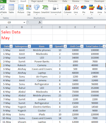
  • On an excel worksheet, you have to select the range of the cells that you want to include in the table.(The cells can be empty or can contain data)
  • On the Insert tab, Click the table in the Tables group.(You can also use shortcut key-CTRL+L or CTRL+T) 
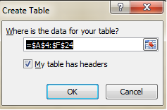
  • Excel automatically select the data for your table or you can add the data to your table.
How to Insert Table in Excel
  • Check "My table has headers" and click OK.
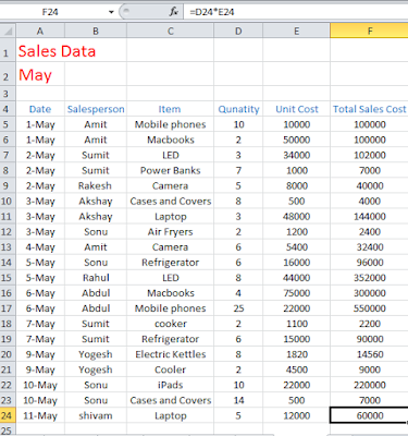
    How to Insert Table in Excel

    Now Excel creates a formatted table for you according to your requirement.

    Sort a Table

    We can sort a table according to our choice. If we want to display the data from lowest to largest or largest to lowest then we can do it very easily by this feature. For that follow some steps:
    • If we want to arrange data from Smallest to Largest then click on the header of that column and then click on Sort Z to A.
    • If we want to arrange data from Largest to Smallest then click on the header of that column and then click on Sort A to Z.
    How to Insert Table in Excel

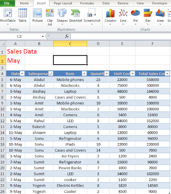
    Here we sort the table according to the name of the salesperson in increasing order of the alphabet.

    Filter a Table

    To format a table, follow some steps :
    • If we want to display any particular data out of whole data then you can apply the filter to the data.
    • For that, you have to click on the header of the particular header and check the particular field according to your requirement.
    How to Insert Table in Excel

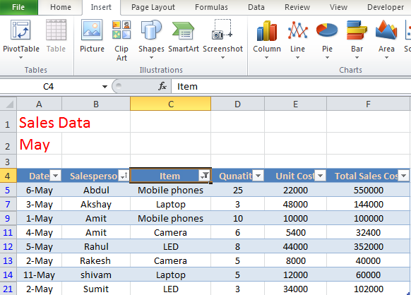
    Here we apply the filter on the Item Column to view only 4 categories like mobile phones, Laptop, Camera and LED out of multiple categories. So by this features, we can apply a filter to view some data according to the requirement.

    Convert a Table to a range of Data

    To convert a table to a range of Data follow some steps:
    • Click any cell in the table.
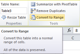
    • On the Design tab, Click Convert to Range from the Tools group.
    How to Insert Table in Excel
    • Now this features to convert the table into a normal range of cells means all of the data is preserved.


    Conclusion:
    Thus, in this post, we focus on how to Insert Table in Excel. Manage the data in the tabular form is the better way for analysis the data and easily access. This feature provides the relevant data according to the customer requirement or we can filter or sort the data. If this post is useful then you can share the post with your friends, colleagues, and relatives. We'll update this post on the regular basis. You can also share this post on facebook, twitter, Google+ or other social media website. If you have any query regarding this post then you can write in the comment section. We'll revert back to you as soon as possible.


    Wednesday, 6 July 2016

    Logical Function in Excel

    Logical Function in Excel: Hello Friends, Today we'll discuss the Logical Function in Excel. MS Excel provides four main logical functions-AND, OR, NOT, and IF. Now some more logical functions are also available to work with the logical value. These functions play an important role when you want to test multiple conditions instead of just one. MS Excel Logical Function returns either TRUE or FALSE as a result when their arguments are evaluated.


    Excel Logical Functions

    There are so many Excel Logical functions available. Here we'll explain some such Functions as below:
    Functions Description
    AND Function Return TRUE if all of its value are TRUE
    OR Function Return TRUE if any argument is TRUE
    NOT Function Reverses the logic of its argument
    IF Function Specifies a logical test to perform
    IFERROR Function Returns a specified value if the formula results in an error otherwise return the result of the formula
    XOR Function Returns a logical exclusive of all arguments

    AND Function

    The AND Function returns TRUE if all its arguments are TRUE and return FALSE if one or more argument are FALSE.

    Formula used: =AND(B1>=20, C1<15)

    Logical Function in Excel

    The formula returns TRUE if a value in cell B2 is greater than or equal to 20 and a value in cell C2 is less than 15 otherwise returns FALSE.

    OR Function

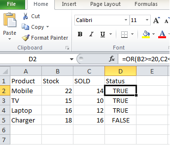
    The OR function returns TRUE if any of its arguments are TRUE and return FALSE if all of its arguments are FALSE.

    Formula Used: =OR(B2>=20, C2<15)

    Logical Function in Excel

    This formula returns TRUE if the value A2>=20 or B2<15 and returns FALSE if all of its argument are FALSE.

    NOT Function

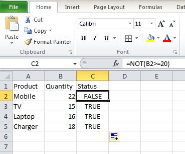
    The NOT function reverses the value of its arguments it means it gives the opposite result.

    Formula Used: =NOT(B2>=20)

    Logical Function in Excel

    This formula returns FALSE if the condition B2>=20 are satisfied otherwise returns TRUE.

    IF Function

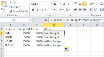
    The IF Function is one of the most useful logical function in MS Excel. It allows you to make comparisons between a value and what you expect. It simply says that If something is TRUE then do something otherwise do something else. IF statements return two values as a result- one value if a condition is TRUE and another value if the condition is FALSE. 

    Formula Used: =IF(C2>B2, "Over Budget", "Within Budget")

    Logical Function in Excel

    This formula returns TRUE if C2<B2 means within Budget and return FALSE means Over Budget if C2>B2.

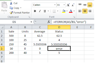
    IFERROR Function

    It returns a specified value if the formula results in an error otherwise return the result of the formula. It is used to trap and handle errors.

    Formula Used: IFERROR(A2/B2,"error")

    Logical Function in Excel

    This formula returns two values either error or result of the formula. It returns TRUE if A2/B2 returns an integer value or result of the formula and it returns FALSE means error if A2/B2 does not return an integer value or result of the formula.

    Conclusion:
    Thus, in this post, you will find the Logical Function in Excel. These functions are very useful in the comparison of multiple data. If you like this post then you can share this post with your friends, colleagues, and relatives. We'll update this post on the regular basis. You can also share this post on facebook, twitter, Google+ or other social media website. If you have any suggestion regarding this post then you can write your views in the comment section. We'll revert back to you as soon as possible.


    Tuesday, 5 July 2016

    How to Protect Excel Sheet with Password

    Protect Excel Sheet with Password: Hello guys, Today we'll discuss that how to Protect Excel Sheet with Password. As We all know that we save all the business data or some important data in excel sheet so it is very important to save excel sheets to prevent other users from viewing, editing, deleting worksheet or any other unauthorized access. You can protect the structure of excel sheet with a password. You should never store sensitive information in an excel spreadsheet without a password. The latest version of MS Excel also provide some more encryption techniques to the more secure spreadsheet.

    Protect Excel sheet with Password

    We store our data in MS Excel spreadsheet because we can protect information with the password and provides the security for the users. There are mainly three ways to protect a workbook or a file as discussed below.

    1. First method to Protect Excel Sheet

    To protect a workbook follow some steps:
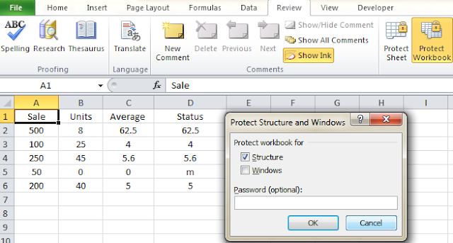
    • Click on Review Tab then clicks on protect workbook.
    • Enter a password in the box.
    How to Protect Excel Sheet with Password
    • Click OK and re-enter the password to confirm.
    • Click OK.

    2. Second method to Protect Excel Sheet

     To protect the MS Excel sheet with password follow some steps as discussed below:
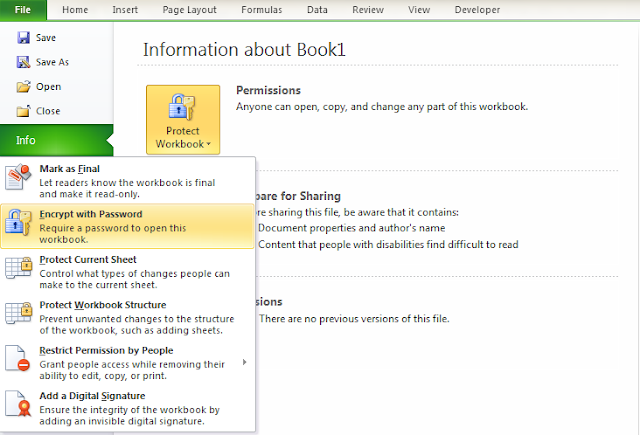
    • Click on the File tab, Click Info option then click on Protect Workbook.
    • Choose Encrypt with Password from the Drop-Down list.
    • Enter a password in the box.
      How to Protect Excel Sheet with Password

    • Click OK and re-enter the Password to confirm.
    • Click OK.

    3. Third Way to Protect a Workbook- Set a Password to allow reading or Modifying

    You can set a Password on the file in two ways-One to open the file as read-only and other to open the file to modify also. Read only access does not provide any changes to a file. If a user needs to be able to modify the file, you will have to share both open and modify the password. For that follow some steps:
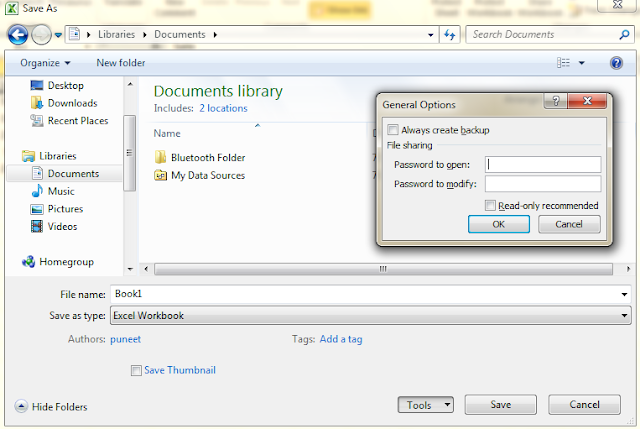
    • Click on File tab and click on Save As option.
    • Click on Browse folder if hide this option.
    • In the Save As Dialog box, click Tools then click on General option.
    How to Protect Excel Sheet with Password

    • Then type the password according to the requirement it means one password to open the file and another to modify the file.
    • Click Save.
    Thus if someone tries to open the file, Excel ask for a password in the first screen. After entering a password a second screen open and ask for a password for modifying the file. Users can click Read Only option if the second password is not available and start viewing the content of the file.


    Conclusion:
    Thus, in this post, You will find that how to Protect Excel Sheet with Password. We can save our useful information to prevent an unauthorized access. If you like this post then you can share this post with your friends, colleagues, and relatives. We'll update this post on a regular basis. You can also share this post on facebook, twitter, Google+ or other social media website. If you have any question regarding this post then you can write in the comment section. We'll revert back to you as soon as possible.
    Monday, 4 July 2016

    How to Use Pivot Table in Excel in 2010

    Pivot Table in Excel 2010: Hello Friends, Today We'll discuss how to Use a Pivot table in Excel 2010.  A pivot table is one of the powerful features of MS Excel. This tutorial will show you how to create a Pivot table in excel to summarize a set of the large dataset according to the requirement. Pivot table report reflects the different view on the same data. You can easily compare data by the Pivot table.For more easily you can also create a Pivot chart to display a summarized data at one place.

    What is a Pivot Table?

    A Pivot table is a report that summarizes,analyze and present a summary of spreadsheet data. It allows you to extract a significance or useful data from a large dataset. It is beneficial when you have a long list of data and basically used for analyzed countless spreadsheet records. We create a Pivot table according to the information and field it means which field to view and how the information should be displayed. There are mainly four things which we can perform using Pivot table in excel:
    • Set up a large dataset in excel so that you can use for a Pivot table.
    • Create a Pivot table with that data.
    • Change the Pivot table report to display different views on same data.
    • Drag,sort and Filter fields according to the requirement.

    Steps for Insert a Pivot Table in MS Excel 2010

    To insert a Pivot table in MS Excel follow some steps:
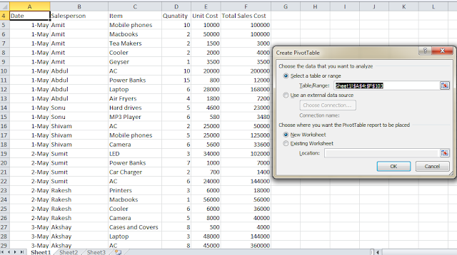
    • Click any cell inside the large dataset.
    • Then on the Insert tab, Click Pivot table. (A dialog box appears in which excel automatically select all the data then choose the location where you want the Pivot table report to be placed)
    How to use Pivot Table in Excel
    • Then click Ok.

      Designing a Pivot Table Layout

      For creating Pivot table Layout follow some steps:
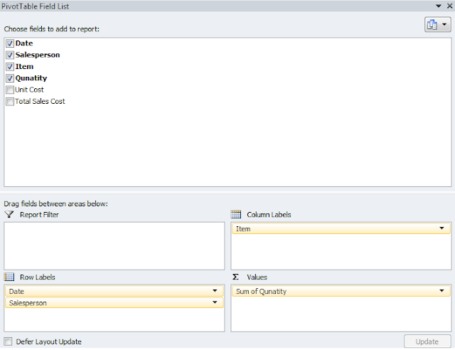
      • When you create a Pivot table then you'll see Pivot Table field list.
      how to use Pivot Table in Excel
      • To create a layout of Pivot table, you first select the Fields then place them in the current location in the field layout area.
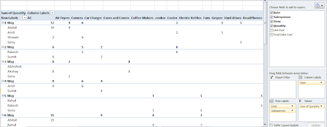
      • Then Pivot table is generated according to the requirement as display below:

      How to Use Pivot Table in Excel in 2010

      Here the Pivot table shows the total number of each product sold by each salesperson on each day.

      Changing a Pivot Table

      You can change a Pivot table to show the table in another way. For that you can follow some steps:
      • Click inside Pivot table report then Pivot table Field list reappear.
      • Change the layout of Pivot table according to the requirement.
      • After these changes, you'll see some reflection on the same data in your Pivot table.
      How to Use Pivot Table in Excel in 2010
      Here the Pivot table shows sold products down the side and name of the salesperson across the top.


      How to Create a Pivot Chart

      To create a Pivot chart follow some necessary steps:

      • Click any cell inside the dataset.
      • On the Insert tab, click Pivot table.
      • Click OK.
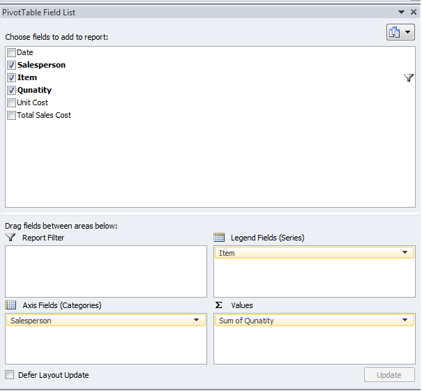
      • You'll see Pivot table Field List, you have choose Fields to add to report and Drag fields between areas like report filter,Legend fields,Axis Fields,and the sum of values.

      How to Use Pivot Table in Excel in 2010

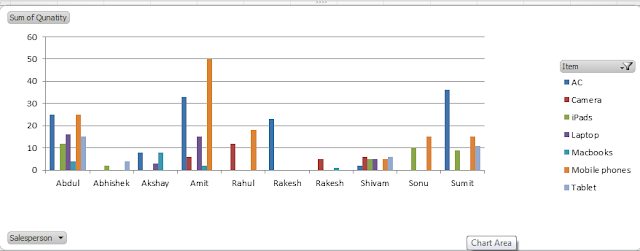
      • Then Pivot chart is generated that is displayed below:
      How to Use Pivot Table in Excel in 2010

      Here Pivot Chart shows the name of the salesperson and the quantity of sold item by each person.


      Conclusion:
      Thus,in this post, we'll discuss that how to use Pivot Table in Excel 2010. Pivot table provides the better way to find the useful information in a minimum time so this tool is very useful in business or in the large organization for prepare the report. If you like this post then you can share this post with your friends, colleagues, and relatives. You find an update on the regular basis. You can also share this post on facebook, twitter, Google+ or other social media website. If you find any issue regarding this post then you can write in the comment section. We'll revert back to you as early as possible.


      How to Calculate Descriptive Statistics in Excel | Data Analysis

      Descriptive Statistics in Excel : Hello friends, in this post, we'll discuss that how to Calculate Descriptive Statistics in Excel. This tutorial useful to show data analysis using an MS Excel spreadsheet program. It is used to the analysis of the data that helps describe or summarize data in a meaningful way. If you want to develop complex Statistical analysis then you can save more time by using Analysis ToolPak. Analysis ToolPak is an excel add-in program that provides data analysis tools for financial, Statistical and engineering data analysis.

      Data Analysis in Excel 2010

      Data Analysis is a process that inspects the data and returns the useful information or summarizes data in a proper manner. Data Analysis functions works on only one worksheet at a time. If you want to use this functions on several worksheets then recalculate for each worksheet.Follow this tutorial to organize a data, use formula and function to calculate Statistical values like mean, standard deviation, standard error or other terms by using MS Excel Analysis ToolPak.

      How to Enable Analysis ToolPak in Excel 2010

      First check Analysis ToolPak tool is available or not in Excel spreadsheet. If this tool is available for access then click on data analysis in the analysis group in the Data tab. If it is not available in current worksheet then we need to activate Analysis ToolPak. For activating this tool follow some steps:
      • First Click on File Tab, click Options then click Add-Ins category.
      • In the bottom view the manage option. Here click on the excel Add-Ins from the drop down list then click on Go.
      • Some Add-ins available so choose Analysis ToolPak out of multiple ToolPak then click Ok.
      • Now Data Analysis option display in the Data Tab.

        Steps For Calculating Descriptive Statistics in Excel

        Descriptive Statistics means a collection of information or summarize data about the observation that have been made.For calculating Descriptive Statistics in excel follow some steps:
        • Click on Data tab then Data analysis from the analysis group.
        • Select Descriptive Statistics and click OK.
        • Select the input Data range.
        • Select Cell for the output.
        • Do not forget to click on summary Statistics.
        • Then click OK for getting the result.

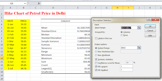
        Hike chart of petrol price in Delhi in last 6 month


        Example: Let we have a Hike chart of petrol price in Delhi in last 6 month and we want to measure some parameters like mean value, standard error value, median, sample variance, kurtosis, skewness, sum, count, minimum value, maximum value or other parameters then we can use Descriptive Statistics functions in MS Excel. Suppose we want to know the minimum and maximum price of the petrol in last six month then this tool is very useful for us.


        Conclusion:
        Thus, in this post, we explain some necessary steps for enabling Analysis ToolPak in Excel. Here we've focused on how to calculate Descriptive Statistics in excel. If you like this post then you can share with friends, colleagues, and relatives. We'll update the information on a regular basis. Please share this post on facebook, twitter, Google+ or other social media website. If you have any suggestion regarding this post then you can write in the comment section. We'll revert back to you as soon as possible. 

        Friday, 1 July 2016

        Salespeople have feelings too…


        A couple of weeks ago, we posted a blog called “We need more sales calls, but it’s not happening.”  The basic premise was this, sales people struggle to produce enough calls because they lack skills, have developed poor habits or just don’t think about how they schedule their time.  I went out of my way to say this…
        "…before I rattle off the reasons, allow me to say I don’t believe sloth has anything to do with the situation.  Lack of skill, sometimes.  Bad habits, probably.  Deliberate laziness, no way."


        I had hoped the article would spark controversy and conversation.  And it did. 

        Since I value the opinion of others and would like the whole of the distributor landscape to give the issue some deeper thought, I am publishing a few of the better stated comments here.

        First, I love the pithiness of this comment…
        “Speaking on behalf of sales people everywhere. I want a supervisor’s advice on sales calls about as much as I want a tax audit.”


        Here’s one that I hear often…
        “I am always amazed how soon after someone moves up from a straight sales role to anything in management they forget what it is like out there on the streets.  All of a sudden they forget all of the totally unreasonable expectations and burdens that their managers put on them and start dumping them on their people.  The best managers I have worked for recognized this and worked hard to keep the level of BS to a minimum.”

        One writer (name withheld to protect the innocent) went on to repudiate a number of my thoughts.  Here they are with very little editing.

        Speaking on the topic of scheduling….
        “Today for example, I had a full day planned 100 miles from my office. One of the counter people even took my premier parking spot. After an hour in a tire shop parking lot talking to my first sales call and fixing some structural issues with his service, my largest customer emails me on what he needs. This is business we have not previously had and will increase market share with him. Best laid plans down the tube.”

        Counting calls to the guard shack as a sales call…
        “I have done those guard shack sales calls. This is what I learned. Who has visited in my industry, the person’s name I need to see, the protocol to get into the gate, visiting hours. One of the most important allies a salesperson can have is the gatekeeper, be it a security guard or receptionist. You have to set up the knock out shot with a jab once in a while.”

        The value of setting appointments…
        “Technical Sales are the best kind of sales. They are asking your advice on what they need. This gives you the ability to customize the BOM to exactly what you have. Technical sales border on design/build and generally have higher margins than standard selling. Sometimes it's just better to freelance than having structured rigidity of scheduling all of your appointments. A little like "Ferris Bueller's Day Off" when you go impromptu you do not know where you will end up.”

        A note from Frank:  Ferris Bueller’s Day Off was one of my
        favorite movies.  For some sick reason I related more to Mr. Rooney, the Dean of Students, who spent his time trying to track down Ferris Bueller.  I hate salespeople who play hooky from work.  Someday ask me about the guy who lost his pager while making sales calls in a remote territory yet his pager turned up on the 11th hole of a local golf course.  My suspicions on him were right.

        Comments about lazy salespeople…
        “I have seen even "Lazy" Salespeople succeed. Much of the time the last person you see is the next person you order from. Some "lazy" salespeople just show up, nothing in hand, no sales pitch, and no plan. They will still succeed at some level.”

        I stand by my original statements.  I believe sellers need to put process into their game.  I totally buy into the sentiment, some sales managers try to micromanage.  However, I also believe some very good journeymen sellers (comment not intended to be sexist), struggle with bad habits, sales slumps and variations in sales activity. 

        I don’t believe in micromanagement, yet many consider even the smallest addition of process to be “dictatorial”.  There are sloppy managers and managers who aren’t operating at the top of their game.  There are even a few sales managers who could serve as poster boys for Dr. Lawrence Peter’s famous principle.  That’s another topic.  However, my advice to distributor leadership has always been to expect heated pushback from your sales team on any change. 

        I believe pushback and resistance from sales teams is a good thing.  Debate is a key ingredient to the development of long term strategy.  Expect it, encourage it.  But once the debate is done, the strategy must be played out with fierce resolve.

        Finally, here is a very important point brought by one of the respondents… I could not agree more.
         “….little of what we do today as sales people affects tomorrow. If your sales are sliding or are flat, that started long before it showed up on any numbers sheet.”

        #truth 

        How to Calculate Total Revenue in MS Excel

        Total Revenue in MS Excel: Hello Friends, Today we'll discuss on how to calculate total revenue in excel. Revenue indicates that overall income that made by the business in the given period of time. Basically, it considers only income which is generated from the business means any deduction, expenditure or any other cost is not included in the Total Revenue. A successful business owner always focuses on total sales revenue for tracking profit/margin in the business. We can easily calculate revenue if we know the price of the good and number of sold goods. 

        Steps For Calculation Total Sales Revenue in MS Excel

        Revenue is the amount that received from selling good or services of a company in a specific period of time. For calculating Revenue, it is necessary to keep records of all the transaction. Revenue can be calculated by a formula :

        Revenue= Price of the Goods * Quantity of the Sold Goods

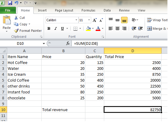
        Let's say you run a Nescafe outlet in a college and you want to calculate total revenue for the month/ quarter or year. First of all, you have proper records of total item sold and price of each product then you can use MS Excel worksheet to calculate total sales revenue. We'll discuss some steps to calculate sales revenue as follow:

        • Go to the excel spreadsheet and type the product's name in the first column A. Here we want to sell Nescafe products then write all the Nescafe products in column A. 
        • After that enter the sale price of the products in cell B. In this cell we write sales prices of all the products.
        How to Calculate Total Revenue in MS Excel

        • Then type the volume of each product in columns C. It means if you sold 125 coffee then write 125 in cell C2 and sold 250 instant food then write 250 in cell C7. 
        • Now enter =B1*C1 in cell D1 till =B8*C8 in cell D8 to calculate total revenue for the particularly given item. 
        • Now calculate total revenue of our escape outlet. For that enter =SUM(D2:D8) and get the total revenue of our sales.

        Steps For Calculation Total Net Income in MS Excel

        Total Net income is calculated by total Revenue and total Expenses. It is the difference between the total revenue and the total expenses. It shows total net income or loss in a financial year in the business. We'll discuss some steps to calculate total net income as follows:
        • First of all, calculate the total Revenue. ( All the steps covered above)
        • Then write all the expenses of a financial year.
        • Then calculate the total expenses using formula.
        • Finally, Calculate total net income or loss using formula.

          How to Calculate Total Revenue in MS Excel

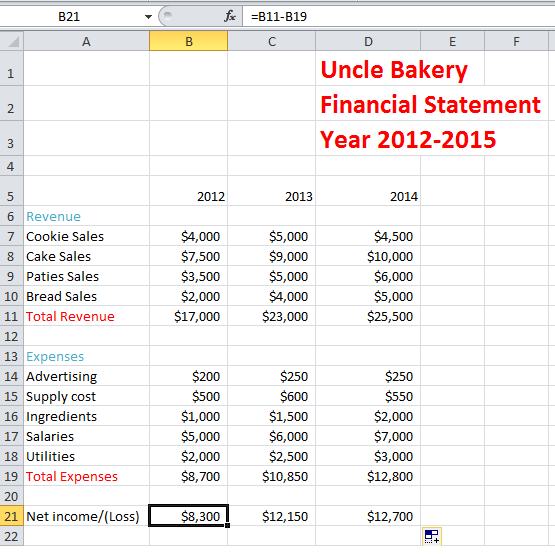
          Example: Here we show the financial balance sheet of  Uncle Bakery. We explain total revenue which gets from the sale of the products(like cookie sales, cake sales, patty sales, and bread sells) and total expenses(like advertising of the product, Supply cost, Ingredients, Salaries,  and Utilities) which used to sell the products. Net income obtained by subtract the total revenue from the total expenses.

          Conclusion:

          Thus, in this post, we explain some step for calculation the total sales revenue in MS Excel. Through this post How to Calculate Total Revenue in MS Excel we want to focus on total income or loss in a financial year. If you like this post then you can share with friends, colleagues, and relatives. We'll update the information on a regular basis. You can also share this post on facebook, twitter, Google+ or other social media website. If you have any suggestion then you can write in comment section. We'll revert back to you as soon as possible.